Sparse Variational Gaussian Process in Multiclass Classification
In this notebook, sparse variational gaussian process model (VGP) is applied to a multiclass classification problem. VGP is easily scalable to large scale dataset.
Background
Consider making inference about a stochastic function \(f\) given a likelihood \(p(y|f)\) and \(N\) observations \(y=\{y_1, y_2, \dots, y_N\}^T\) at observation index points \(X=\{x_1, x_2, \dots, x_N\}^T\). Place a GP prior on \(f\): \(p(f) \sim N(f|m(X), K(X, X))\). The joint distribution of data and latent stochastic function is
\[p(y, f) = \prod_{i=1}^{N}p(y_i|f_i)N(f|m(X), K(X, X)) \tag{1}\]
\(\qquad\) The main interest is the posterior over the function values given the observations \(p(f|y)\). The posterior is intractable when the likelihood \(p(y|f)\) is non-Gaussian, which is often the case in classification problems; and the computational complexity is \(O(N^3)\) due to the inversion of \(K_{X, X}\), which is also intractable for large dataset.
\(\qquad\) To reduce the computational complexity, \(M << N\) inducing index points \(Z=\{z_1, z_2, \dots, z_M\}^T\) and inducing variables \(u=f(Z)\) are introduced. Assuming a GP prior on the joint density \(p(f, u)\), \[p(f, u) = N\begin{pmatrix} \begin{bmatrix} f \\ u\end{bmatrix}| \begin{bmatrix} m(X) \\ m(Z)\end{bmatrix}, \begin{bmatrix} K(X, X) & K(X, Z) \\ K(Z, X) & K(Z, Z)\end{bmatrix}\end{pmatrix},\] and a GP prior on \(u\) \[p(u) = N(u|m(Z), K(Z, Z)),\] the conditional of \(f\) is \(p(f|u) = N(f|\mu, \Sigma)\), where for \(i, j = 1, \dots, N\)
\[[\mu]_i = m(x_i) + \alpha(x_i)^T(u-m(Z)), \tag{2}\]
\[[\Sigma]_{ij} = K(x_i, x_j) - \alpha(x_i)^T K(Z, Z)\alpha(x_j), \tag{3}\] where \(\alpha(x_i) = K(Z, Z)^{-1}K(Z, x_i)\), and the joint density of \(y, f, u\) becomes
\[p(y, f, u) = p(f|u; X, Z)p(u; Z)\prod_{i=1}^{N}p(y_i|f_i)\]
\(\qquad\) The goal is still finding the posterior of the function values \(f\), however, the likelihood \(p(y_i|f_i)\) is not Gaussian, so no closed-form solution for the posterior of \(f\). Therefore, a variational posterior is used to solve the difficulty.
\(\qquad\) Replacing the posterior \(p(u|y)\) by an arbitrary full-rank Gaussian distribution \(q(u)\) [Hensman et al. (2013)], then the variational posterior for \(y\) and \(u\) jointly becomes
\[q(f, u; X, Z) = p(f|u; X, Z)q(u), \tag{4}\]
\[\mbox{where } q(u) \sim N(\mathbf{m}, \mathbf{S})\]
\(\mathbf{m}, \mathbf{S}\) are parameters to be chosen by optimizing an evidence lower bound (ELBO).
\(\qquad\) Since both \(p(f|u; X, Z)q(u)\) are Gaussian, the marginal variational posterior of \(f\) can be computed analytically
\[q(f|\mathbf{m}, \mathbf{S}; X, Z) = \int p(f|u; X, Z)q(u) du \sim N(\tilde{\mu}, \tilde{\Sigma}) \tag{5}\]
with \([\tilde{\mu}]_i = \mu_{\mathbf{m}, Z}(x_i), [\tilde{\Sigma}]_{ij} = \Sigma_{\mathbf{S}, Z}(x_i, x_j)\), and
\[\mu_{m, Z}(x_i) = m(x_i)+\alpha(x_i)^T(\mathbf{m}-m(Z)) \tag{6}\] \[\Sigma_{S, Z}(x_i, x_j) = K(x_i, x_j) - \alpha(x_i)^T[K(Z, Z) - \mathbf{S}]\alpha(x_j) \tag{7}\]
\(\qquad\) The variation parameters \(Z, \mathbf{m}, \mathbf{S}\) in \(q(f|\mathbf{m}, \mathbf{S}; X, Z)\) are determined by maximizing the lower bound
\[L = \sum_{i=1}^N \mathbb{E}_{q(f_i|\mathbf{m}, \mathbf{S}; X, Z)}[logp(y_i|f_i)] - KL[q(u)|| p(u)], \tag{8}\]
where the expected log-likelihood can be computed with Gauss–Hermite quadrature.
\(\qquad\) The variational posterior is given as \(q(f)\) in (5). To make predictions for a set of test index points \(X^*\), the new latent function values \(f^*\) is approximated by
\[\begin{equation}\begin{array}{rcl}p(f^*|y) &=& \int p(f^*|f, u)p(f, u|y) df du\\ &\approx& \int p(f^*|f, u)p(f|u)q(u)df du \\ &=& \int p(f^*|u)q(u) du \\ &=& q(f^*)\end{array}\end{equation}\]
where the last line is following (5), (6) and (7) by replacing \(x_i\) by \(x_i^*\).
\(\qquad\) With the variational posterior in (5), the predictive mean and variance of \(y^*\) are computed as
\[\hat{y}^* = \mathbb{E}(y^*) = \int\int y^* p(y^*|f^*)q(f^*) df^* dy^* \tag{9}\] \[\hat{\mathbb{V}}(y^*) = \int\int y^{*2} p(y^*|f^*)q(f^*) df^* dy^* \tag{10}\]
References
[1]: Titsias, M. “Variational Model Selection for Sparse Gaussian Process Regression”, 2009. http://proceedings.mlr.press/v5/titsias09a/titsias09a.pdf
[2]: Hensman, J., Lawrence, N. “Gaussian Processes for Big Data”, 2013. https://arxiv.org/abs/1309.6835
[3]: Salimbeni, H. and Deisenroth, M. “Doubly stochastic variational inference for deep Gaussian processes.” Advances in Neural Information Processing Systems. 2017. https://arxiv.org/pdf/1705.08933.pdf
Imports
import matplotlib.pyplot as plt
import numpy as np
import tensorflow.compat.v2 as tf
import tensorflow_probability as tfp
import pandas as pd
from sklearn.preprocessing import LabelEncoder
from sklearn.model_selection import train_test_split
from scipy.cluster.vq import kmeans2

tf.enable_v2_behavior()

tfb = tfp.bijectors
tfd = tfp.distributions
tfk = tfp.math.psd_kernels

dtype = np.float64
Load Glass Data
A standard imbalanced machine learning dataset referred to as the “Glass Identification” dataset, or simply “glass”.
The dataset describes the chemical properties of glass and involves classifying samples of glass using their chemical properties as one of six classes. The dataset was credited to Vina Spiehler in 1987.
#!wget https://raw.githubusercontent.com/jbrownlee/Datasets/master/glass.csvdata = pd.read_csv('glass.csv', header=None)
data = data.values
X = data[:,0:9].astype(dtype)
Y = data[:,9]
encoder = LabelEncoder()
encoder.fit(Y)
encoded_Y = encoder.transform(Y)
encoded_Y = encoded_Y.astype(dtype)
num_outputs = 6
X_train, X_test, y_train, y_test = train_test_split(X, encoded_Y, test_size=0.2, random_state=42)
print(X_train.shape, X_test.shape, encoded_Y.shape)(171, 9) (43, 9) (214,)Defining Trainable Variables in VGP
- Using kmeans to initialize 30 representative
inducing_index_points\(Z\) and make them learnable variable
num_inducing_points_ = 30
inducing_index_points_init = kmeans2(X_train, num_inducing_points_, minit="points")[0] #50, 60
inducing_index_points = tf.Variable(inducing_index_points_init, dtype=dtype, name='inducing_index_points')- Initializing RBF kernel and kernel parameters, which are
amplitudeandlength_scale(the same length scale is used for all \(X\) columns) - Initializing the variational mean and covariance \(\mathbf{m}, \mathbf{S}\) in \(q(u)\)
amplitude = tfp.util.TransformedVariable(
    1., tfb.Softplus(), dtype=dtype, name='amplitude')
length_scale = tfp.util.TransformedVariable(
    1., tfb.Softplus(), dtype=dtype, name='length_scale')
kernel = tfk.ExponentiatedQuadratic(amplitude=amplitude, length_scale=length_scale)

observation_noise_variance = tfp.util.TransformedVariable(1., tfb.Softplus(), dtype=dtype, name='observation_noise_variance')

variational_inducing_observations_loc = tf.Variable(np.zeros([num_outputs, num_inducing_points_], dtype=dtype), name='variational_inducing_observations_loc')

Ku = kernel.matrix(inducing_index_points, inducing_index_points)
variational_inducing_observations_scale_init = np.linalg.cholesky(Ku + np.eye(num_inducing_points_)*1e-6)
variational_inducing_observations_scale = tf.Variable(np.tile(variational_inducing_observations_scale_init[None, :, :], [num_outputs, 1, 1]),
name='variational_inducing_observations_scale')- Defining log probability. For multiclass classification, Categorical distribution is used. The
observationsis a flat array of batch size; since the expected log likelihood in VGP is approximated by Gauss–Hermite quadrature, the input logits is reshaped to (quadrature_size, batch_size, num_outputs) to adapt to thesparse_softmax_cross_entropy_with_logitsinlog_prob
def log_prob(observations, f):
    #f is (6, 20, 64)
    berns = tfd.Independent(tfd.Categorical(logits=tf.transpose(f, perm=[1,2,0])), 1) #(20, 64, 6), n_quadrature, bs, n_outputs
    return berns.log_prob(observations) #sparse_softmax_cross_entropy_with_logits: have logits of shape [batch_size, num_classes] and have labels of shape [batch_size]
Constructing Model and Training
vgp = tfd.VariationalGaussianProcess(
    kernel,
    index_points=X_test,
    inducing_index_points=inducing_index_points,
    variational_inducing_observations_loc=variational_inducing_observations_loc, #TensorShape([6, 30])
    variational_inducing_observations_scale=variational_inducing_observations_scale, #TensorShape([6, 30, 30])
    observation_noise_variance=observation_noise_variance)
batch_size = 64
optimizer = tf.optimizers.Adam(learning_rate=.01)
@tf.function
def optimize(x_train_batch, y_train_batch):
with tf.GradientTape() as tape:
# Create the loss function we want to optimize.
recon = vgp.surrogate_posterior_expected_log_likelihood(
observations=y_train_batch,
observation_index_points=x_train_batch,
log_likelihood_fn=log_prob,
quadrature_size=20)
elbo = -tf.reduce_sum(recon) + tf.reduce_sum(vgp.surrogate_posterior_kl_divergence_prior())
grads = tape.gradient(elbo, vgp.trainable_variables)
optimizer.apply_gradients(zip(grads, vgp.trainable_variables))
return elboTraining by Batch
num_iters = 1200
num_logs = 10
num_training_points_ = X_train.shape[0]

for i in range(num_iters):
    batch_idxs = np.random.randint(num_training_points_, size=[batch_size])
    x_train_batch = X_train[batch_idxs, ...]
    y_train_batch = y_train[batch_idxs]
    loss = optimize(x_train_batch, y_train_batch)

    if i % (num_iters / num_logs) == 0 or i + 1 == num_iters:
        print(i, loss.numpy())
WARNING:tensorflow:From /rhome/lp/.conda/envs/ipykernel_py2/lib/python3.8/site-packages/tensorflow/python/ops/linalg/linear_operator_full_matrix.py:142: calling LinearOperator.__init__ (from tensorflow.python.ops.linalg.linear_operator) with graph_parents is deprecated and will be removed in a future version.
Instructions for updating:
Do not pass `graph_parents`.  They will  no longer be used.
0 114.67260603059553
120 68.34762534248783
240 64.21088822088196
360 57.34725658089357
480 55.54024567522668
600 55.44484420146989
720 47.751929090335935
840 51.43769578785385
960 46.757460639624206
1080 45.57974099864305
1199 34.62597956776342
Computing the Predictive Mean and Variance
To compute the predictive mean and variance for a set of new \(X^*\), the predict_mean_and_var from gpflow is used to compute (9) and (10).
from gpflow.likelihoods.multiclass import Softmax

Fmu = tf.cast(tf.transpose(vgp.mean()), tf.float32) #TensorShape([6, 43])
Fvar = tf.cast(tf.transpose(vgp.variance()), tf.float32)##TensorShape([6, 43])

S = Softmax(num_outputs)
m, v = S.predict_mean_and_var(Fmu, Fvar) #shape=(43, 6)
Results and Plots
acc =np.mean(np.argmax(m, 1).astype(int) == y_test.astype(int))
print("Multiclass classification accuracy for {} is {}".format(num_outputs, acc))
Multiclass classification accuracy for 6 is 0.6744186046511628indices = np.argmax(m, 1)
v_ = tf.reduce_sum(tf.one_hot(indices, 6)*v, 1)
print("Multiclass classification variances for {} is {}".format(num_outputs, v_))Multiclass classification variances for 6 is [0.21738583 0.21815017 0.18933281 0.22934248 0.21277648 0.16272718
0.22080968 0.20925453 0.24283622 0.23389922 0.18182059 0.17588708
0.22748089 0.21455643 0.2155985 0.20811221 0.17323363 0.22754371
0.2092959 0.1684241 0.20327246 0.19117251 0.23838614 0.23942412
0.2244384 0.1978951 0.2334285 0.23561463 0.19514483 0.23224472
0.20528135 0.22660583 0.20674482 0.21365893 0.22525424 0.20758402
0.17756931 0.23329203 0.23498446 0.21907398 0.16997713 0.22914468
0.22700277]from sklearn.decomposition import PCA
pca = PCA(n_components=1)
X_test_pca = pca.fit_transform(X_test)
y_preds = np.argmax(m, 1).astype(int)
y_sd = (v_)**0.5Each dot is the predicted class for each \[x_i^*\], and the error bar is one sd of \(y_i^*\). If the a dot and a cross overlap, this is a correct prediction.
plt.figure(figsize=(15, 5))
plt.scatter(X_test_pca, y_test,
            marker='x', s=50, c=y_test, zorder=10)

plt.errorbar(X_test_pca, y_preds, yerr=y_sd, fmt='o', capthick=1, label='Predidtion', alpha=0.5)
plt.legend(loc='upper right')
plt.ylabel('6 Classes of Glasses')
plt.xlabel('X_test_pca')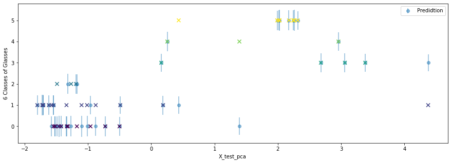
Author Luyao Peng
LastMod 2020-11-05