R Package “regrrr”: Compiling and Visualizing Regression Results
Contents
This is an R package “regrrr” on Cran I coauthored with Rui Yang.
In strategy/management research, we always need to compile the regression results into the publishable format and sometimes plot the moderating effects. This package does the job.
Here is the quickstart guide.
Installation
To install from CRAN:
install.packages("regrrr")
library(regrrr)
You can also use devtools to install the latest development version:
devtools::install_github("raykyang/regrrr")
library(regrrr)
Examples
compile the correlation table
library(regrrr)## Warning: package 'regrrr' was built under R version 3.5.2data(mtcars)
m0 <- lm(mpg ~ vs + carb + hp + wt, data = mtcars)
m1 <- update(m0, . ~ . + wt * hp)
m2 <- update(m1, . ~ . + wt * vs)
cor.table(data = m2$model)## Mean S.D. 1 2 3 4 5
## 1.mpg 20.09 6.03 1.00
## 2.vs 0.44 0.50 0.66 1.00
## 3.carb 2.81 1.62 -0.55 -0.57 1.00
## 4.hp 146.69 68.56 -0.78 -0.72 0.75 1.00
## 5.wt 3.22 0.98 -0.87 -0.55 0.43 0.66 1.00compile the regression table
regression_table <- rbind(
combine_long_tab(to_long_tab(summary(m0)$coef),
                 to_long_tab(summary(m1)$coef),
                 to_long_tab(summary(m2)$coef)),
compare_models(m0, m1, m2))
rownames(regression_table) <- NULL
print(regression_table)
## Variables Model 0 Model 1 Model 2
## 1 (Intercept) 35.435*** 48.157*** 46.698***
## 2 (2.503) (4.097) (9.272)
## 3 vs 1.353 1.077 2.171
## 4 (1.382) (1.152) (6.320)
## 5 carb -0.057 -0.043 -0.009
## 6 (0.449) (0.374) (0.426)
## 7 hp -0.024† -0.113*** -0.107*
## 8 (0.014) (0.027) (0.044)
## 9 wt -3.792*** -8.071*** -7.594*
## 10 (0.658) (1.307) (3.016)
## 11 hp:wt 0.027** 0.025†
## 12 (0.008) (0.015)
## 13 vs:wt -0.367
## 14 (2.081)
## 15 R_squared 0.833 0.889 0.889
## 16 Adj_R_squared 0.808 0.867 0.862
## 17 Delta_F 12.517** 0.031plot the moderating effect
plot_effect(reg.coef = summary(m2)$coefficients, data = mtcars, model = m2,
            x_var.name = "wt", y_var.name = "mpg", moderator.name = "hp",
            confidence_interval = TRUE,  CI_Ribbon = FALSE,
            xlab = "Weight", ylab = "MPG", moderator.lab = "Horsepower") +
ggplot2::theme(text=ggplot2::element_text(family="Times New Roman", size = 16))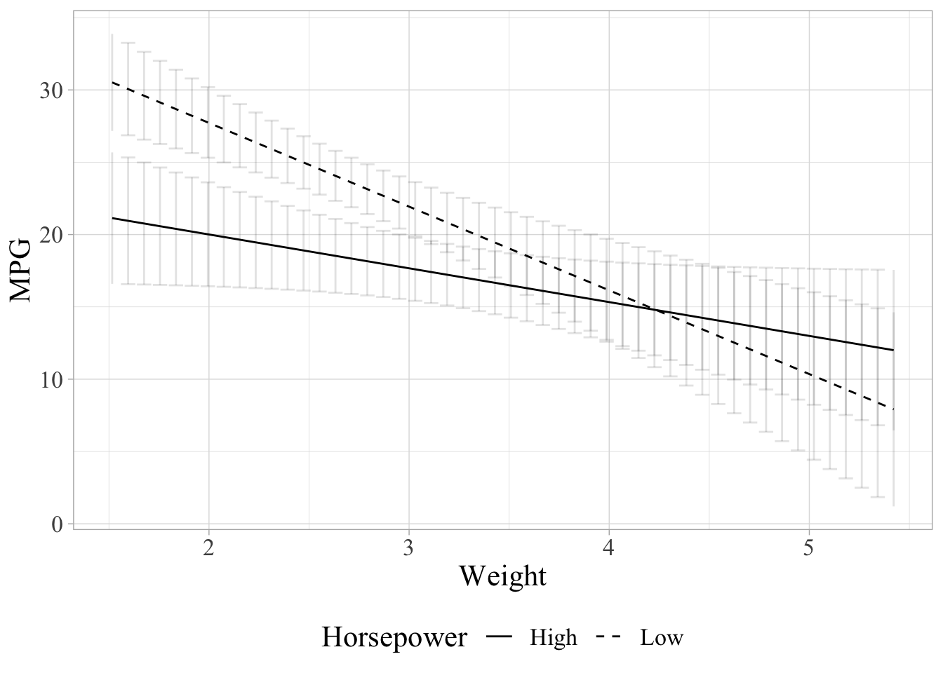
As you can see from the last line of code, the plot is customizable using “ggplot2”. There are a couple of other functions. Please see the reference manual on R documentation for details.
Author Luyao Peng
LastMod 2019-03-10