Correspondence Between Infinitely Wide Deep Neural Networks and Gaussian Process
Contents
Equivalency between Gaussian Process and DNNs
Previous studies have shown the equivalency between Gaussian Process (GP) [1] and infinitely wide fully-connected Neural Networks (NNs) [2][4], which implies that if we choose a fully-connected NN with infinite width, the function computed by the NN is equivalent to a function drawn from a GP under appropriate statistical assumptions. The analytic forms of GP kernel for DNNs were also subsequentially developed.
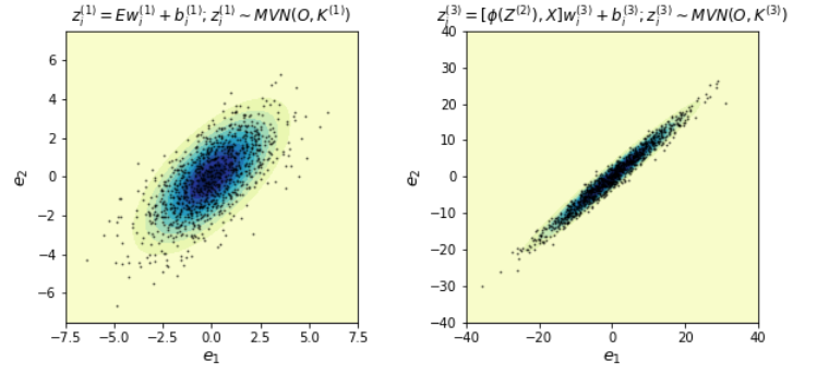
The following figure shows the consistency between the theoretical GP (contour rings) and the sampled \(z_i\) at the initial layer (left) and the third layer (right) in a DNN. Note the kernel \(K\) in MVN is computed based on the method in [2].
We can also show the correspondence theoretically.
Consider a fully-connected feed-forward NN with \(L\) layers. Let \(\phi\) be pointwise nonlinear function, \(X^l\) and \(y\) denote the input features at the \(l\)th layer and the target, respectively, \(z_i^l\) is the ith post-linear transformation component at the \(l\)th layer, \(i=1, \dots, n^l\), \(Z^l=[z_1^l, \dots, z_{n^l}^l]\), \(n^l\) is the width at the \(l\)th layer, \(w_i^l\) and \(b_i^l\) are the weight and bias vectors for \(z_i^l\), then
\[\begin{equation}\label{eq:1} \begin{aligned}[l] z_i^0&=X^0 w_i^0+b_i^0\\ z_i^1 &= X^1w_i^1+b_i^1\\ &\qquad \vdots\\ \quad z_i^{L-1} &= X^{L-1}w_i^{L-1}+b_i^{L-1} \quad\\ \quad z^{L} &=X^{L}w^{L}+b^{L}\\ \mbox{prediction:}\quad y &= z^L+\epsilon\\ \end{aligned} \begin{aligned}[c] X^1 &= \phi(Z^0) \\ X^2 &= \phi(Z^1)\\ &\quad\vdots\\ X^L &= \phi(Z^{L-1})\\ &\quad\\ &\quad\\ \end{aligned} \end{equation}\]
If we assume \(w_i^{l} \stackrel{iid}{\sim} MVN(0, \frac{\sigma_w^{2}}{n^l}I),b_i^{l}\stackrel{iid}{\sim} MVN(0, \sigma_b^{2}I)\), then
Layer 0: Each element in layer 0 is \(z_{ki}^0 = \mathlarger{\sum}_{j=1}^{n^0} x_{kj}w_{ji}^0+b_{ki}\), which is a sum of iid random variables for \(k=1, \dots, N\). If \(n^0 \rightarrow \infty\), we have \(z_i^0 \stackrel{iid}{\dot{\sim}} MVN(0, \frac{\sigma_w^2}{n^0}XX'+\sigma_b^2I)\) by Central Limit Theorem (CLT), where the \(\cdot\) indicates ‘approximately’.
Layer 1-L: Each element in \(z_{i}^l\) is also a sum of iid random variables, where \(z_i^l \stackrel{iid}{\dot{\sim}} MVN\left(0, K^l(X^l, X^{l})\right)\), where
\[\begin{equation}\label{eq:2} K^l(X^l, X^{l}) = \frac{\sigma_w^2}{n^l}\mathbb{E}\left[\phi(X^{l-1})\phi(X^{l-1})'\right]+\sigma_b^2I, [2] \end{equation}\]
Advantages of GPDNN:
- GPDNNs are essentially a DNN based on bayesian method to weight the final predictions by the posterior probabilities of the parameters, weights and bias in each layer, which implies the ensemble learning nature of GPDNN, because it takes into account of the probabilities of all possible values of weights and bias parameters. This is important in reducing the prediction variance, achieving a stable predictions and avoid overfitting problems that exist in deep learning techniques.
- The gaussian process regression or classification model [1] can be implemented after driving the GP forms of a DNN, which yields closed-form predictions/ This saves the training time dramatically compared to deep learning methods.
- GPDNNs is scalable to large-scale data by using gpytorch library to solve Cholesky Decomposition in parallel.
References:
Rasmussen and Williams, 2006: Gaussian Processes for Machine Learning
Lee et al., 2018: Deep Neural Networks as Gaussian Processes
Zhang et al., 2019: Sequential Gaussian Processes for Online Learning of Nonstationary Functions
Williams, 1997: Computing with infinite networks
Author Luyao Peng
LastMod 2019-12-25