Empirical Bayesian Neural Network
Contents
Bayesian approaches to neural networks (BNNs) training [1] have gained increased popularity in NLP community due to its merits of scalability, providing inference uncertainty, and its ensemble learning nature. Despite those features, BNNs are sensitive to the choice of prior and require to tune the parameters in the prior distribution assumed for model weights and biases [2][3]. Sensitivity to the prior and its initialization makes BNNs difficult to train in practice.
We apply the empirical bayesian neural network (EBNNs) proposed by [3] and the method of quantifying the classification uncertainty [12] to the named entity recognition, a classification task in NLP community and compare five common NLP models in terms of multi-class classification accuracy and training time.
Bayesian Neural Networks
For BNNs, they follow windowed input and a feed-forward two-layer neural network (FNNs) architecture. The difference is that all the weights in BNNs are represented by probability distributions over their possible values, while all the weights have fixed values to be learned in FNNs [1]. Define \(w_{ij}\) as a single weight in the model parameters \(\mathbf{W}, \mathbf{U}, \mathbf{b}_1, \mathbf{b}_2\), and \(\mu_{ij}, \sigma_{ij}\) as the mean and scale for \(w_{ij}\), then the window-based BNNs can be expressed as
\[ \begin{aligned} \mathbf{e}_t &= [\mathbf{x}_{t-w}\mathbf{E}, \dots, \mathbf{x}_{t}\mathbf{E}, \dots, \mathbf{x}_{t+w}\mathbf{E}]\\ \mathbf{h_t} &= \phi(\mathbf{e}_t\mathbf{W}+\mathbf{b}_2)\\ \hat{\mathbf{y}_t} &=softmax(\mathbf{h}_t\mathbf{U}+\mathbf{b}_2)\\ &\mbox{where } w_{ij} \sim N(\mu_{ij}, \sigma_{ij}) \quad (1)\\ \end{aligned} \] The weights in BNNs are assumed to be independent, meaning that each weight has its own mean and scale.
Variational Bayesian Neural Networks
Let \(\mathbf{D} = \left\{X, y\right\}, X\in \mathbb{R}^{N\times D}, y\in \mathbb{R}^{N\times 1}\) be the dataset containing windowed input matrix and the associate target vector in the named entity recognition, let denote the weights and biases in a BNN, it is assumed that \(p(Y|\mathbf{w}, X)\) is a categorical distribution conditioned on , the goal of model training is to find out \(p(y|X) = \int_\mathbf{w}p(y|\mathbf{w}, X)p(\mathbf{w|\mathbf{D}})d\mathbf{w}\) , which is the probability of given by integrating our all possible \(\mathbf{w}\).
To achieve this goal, one needs to find out the posterior distribution of \(\mathbf{w}\), i.e., \(p(\mathbf{w}| \mathbf{D})\). Since the likelihood distribution \(p(y|\mathbf{w}, X)\) is not Gaussian in classification problem, the analytic form of the posterior \(p(\mathbf{w}| \mathbf{D})\) is not tractable. To address this problem, a variational approach [8][9][10] is developed by introducing a variational distribution \(q(\mathbf{w}| \mathbf{\theta})\) within a known distribution family with parameters \(\mathbf{\theta} = (\mathbf{\mu}_q, \Sigma_{q})\) to approximate the true posterior \(p(\mathbf{w}| \mathbf{D})\). The approximation is learned by minimizing the Kullback-Leibler divergence (KL) between \(q(\mathbf{w}| \mathbf{\theta})\) and \(p(\mathbf{w}| \mathbf{D})\) with respect to . Therefore, in BNNs, the objective function to minimize is
\[ \begin{aligned} KL(q(\mathbf{w}| \mathbf{\theta}) || p(\mathbf{w}|\mathbf{D})) &= \int_{w} q(\mathbf{w}| \mathbf{\theta})log\frac{q(\mathbf{w}| \mathbf{\theta})}{p(\mathbf{w}|\mathbf{D}))}dw\\ & = \int_{w} q(\mathbf{w}| \mathbf{\theta})log\left(\frac{q(\mathbf{w}| \mathbf{\theta})}{p(y|\mathbf{w}, X))p(\mathbf{w})}p(y|X)\right)dw\\ & = KL[q(\mathbf{w}| \mathbf{\theta}) || p(\mathbf{w})]-\mathbb{E}_{q(\mathbf{w}|\theta)}[logp(y|\mathbf{w}, X)] \quad (2)\\ & \qquad\qquad\qquad\qquad\qquad\qquad+log[p(y|X)]\\ \end{aligned} \] Since \(log[p(y|X)]\) doesn’t depend on \(\mathbf{w}\), minimizing \(KL(q(\mathbf{w}|\mathbf{\theta}) || p(\mathbf{w}|\mathbf{D}))\) s equivalent to minimize the first two terms on the right hand side, which is called the variational free energy \(\mathcal{F}(\mathbf{D}, \mathbf{\theta})\),
\[ \begin{aligned} \mathcal{F}(\mathbf{D}, \mathbf{\theta}) = KL[q(\mathbf{w}| \mathbf{\theta}) || p(\mathbf{w})]-\mathbb{E}_{q(\mathbf{w}|\theta)}[logp(y|\mathbf{w}, X)] \qquad (3) \end{aligned} \]
People often maximize the negative of \(\mathcal{F}(\mathbf{D}, \mathbf{\theta})\), which is called the evidence lower bound \(\mathcal{L}(\mathbf{D}, \mathbf{\theta} )\),
\[ \begin{aligned} \mathcal{L}(\mathbf{D}, \mathbf{\theta})& = \mathbb{E}_{q(\mathbf{w}| \mathbf{\theta})}[logp(y|\mathbf{w}, X)]-KL[q(\mathbf{w}| \mathbf{\theta}) || p(\mathbf{w})]\\ &=\mathbb{E}_{q(\mathbf{w}| \mathbf{\theta})}[logp(y|\mathbf{w}, X)] - \mathbb{E}_{q(\mathbf{w}| \mathbf{\theta})}logq(\mathbf{w}|\theta ) + \mathbb{E}_{q(\mathbf{w}| \mathbf{\theta})}log p(\mathbf{w}) \quad (4) \end{aligned} \]
Since BNNs involves nonlinear transformation \(\phi\)n each layer, each \(\mathbb{E}\) term in Equation (4) is intractable, monte carlo (MC) can be used to estimate \(\mathbb{E}\) by sampling \(\mathbf{w}\) from \(q(\mathbf{w}|\theta)\) each epoch to maximize \(\mathcal{L}(\mathbf{D}, \mathbf{\theta} )\),
\[ \mathcal{L}(\mathbf{D}, \theta) \approx \frac{1}{S}\sum_{s=1}^{S}log p\left(y|\mathbf{w}^{(s)},\mathbf{x}\right) - \frac{1}{S}\sum_{s=1}^{S}log q(\mathbf{w}^{(s)}|\theta)+\frac{1}{S}\sum_{s=1}^{S} p(\mathbf{w}^{(s)}) \quad (5) \] Maximizing \(\mathcal{L}(\mathbf{D}, \mathbf{\theta} )\) encourages the model to find \(\theta\) such that \(q(\mathbf{w}|\mathbf{\theta})\) is closest to \(p(\mathbf{w}| \mathbf{D})\) within a distribution family, then it can be assumed that \(w_{ij} \sim q(\mathbf{w}|\mathbf{\theta})\) independently.
Empirical Variational Bayesian Neural Networks
The Model
Equation (2) requires us to define the prior distribution \(p(\mathbf{w})\), for which there is usually little intuition to select the prior parameters in practice, [3] proposes to parameterize the prior \(p(\mathbf{w})\) hierarchically as \(p(w_{ij}|s)\sim N(0, s)\) where \(s\sim \mbox{Inv-Gamma}(\alpha, \beta)\), then the \(KL(q(\mathbf{w}| \mathbf{\theta}) || p(\mathbf{w}|\mathbf{D}))\) in Equation (2) becomes
\[ \begin{aligned} KL(q(\mathbf{w}| \mathbf{\theta}) || p(\mathbf{w}|\mathbf{D})) = KL[q(\mathbf{w}| \mathbf{\theta}) || p(\mathbf{w}|s)]&-log p(s) -\mathbb{E}_{q(\mathbf{w}|\mathbf{D}), \mathbf{\theta}}[logp(y|\mathbf{w}, X)] \\ & +log[p(y|X)] \qquad\qquad (6) \end{aligned} \] Under independence assumption of each weight, and both \(q(\mathbf{w}|\theta) \mbox{ and } p(\mathbf{w}|s)\) in Equation (6) are Gaussians with means and covariances \(\mathbf{\mu}_q, \Sigma_{q}=\sigma_{ij}\mathbf{I}, \mathbf{\mu}_p=\mathbf{0}, \Sigma_{p}=s\mathbf{I}\) from [3][10], it can be written as
\[ \begin{aligned} KL[q(\mathbf{w}| \mathbf{\theta}) || p(\mathbf{w}|s)] &= \frac{1}{2} \left(log\frac{|\Sigma_p|}{|\Sigma_q|}-D+Tr(\Sigma_p^{-1}\Sigma_q)+(\mu_p-\mu_q)^{T}\Sigma_p^{-1}(\mu_p-\mu_q)\right)\\ & = \frac{1}{2} \left(log\frac{N_ws}{|\Sigma_q|}-D+Tr(s^{-1}\Sigma_q)+s^{-1}\mu_q^{T}\mu_q)\right) \qquad (7) \end{aligned} \]
Taking derivative of \(KL[q(\mathbf{w}| \mathbf{\theta})\) with respect to \(s\), we have
\[ \frac{dKL(q||p)}{ds} = \frac{N_w}{2s}-\frac{1}{2s^2}Tr(\Sigma_q+\mu_q\mu_q^{T}) \qquad (8) \]
Taking derivative of \(log p(s)\) with respect to \(s\), we have
\[ \begin{aligned} \frac{dlog p(s)}{ds} &= \frac{d}{ds}log\frac{\beta^\alpha}{\Gamma^\alpha}-(\alpha+1)logs-\beta\frac{1}{s}\\ & = -(\alpha+1)\frac{1}{s}+\frac{\beta}{s^2} \qquad\qquad\quad (9) \end{aligned} \] Having Equation (9) minus Equation (10), and let the result equal to 0, we can solve for \(s\) \[ \hat{s} = \frac{Tr(\sigma_{ij}\mathbf{I}+\mu_q\mu_q^{T})+2\beta}{N_w+2\alpha+2} \qquad\qquad (10) \] Plugging \(\hat{s}\) into Equation (6), it becomes a function of \(\theta\), we can take gradients with respect to \(\theta\) in Equation (6) to learn \(\theta\) empirically. Equation (10) corresponds to the code
      m = tf.cast(mu.shape[0], dtype='float32')
      S = tf.reduce_sum(sigma + mu * mu, axis=0)
      m_plus_2alpha_plus_2 = m + 2.0 * self.prior_alpha + 2.0
      S_plus_2beta = S + 2.0 * self.prior_beta
      s_hat = S_plus_2beta / m_plus_2alpha_plus_2
The Optimization Procedures
The optimization procedure of EBNN is the following:
Initialize \(\theta = \mu_{ij}, \sigma_{ij} \mbox{ in } q(w_{ij}|\theta)\) randomly and independently for each weight in BNN model;
Build BNN model based on Equation (1), using re-parameterization trick to compute and is independent [1];
With the initialized \(\theta\) in step (1) and define a broad inv-gamma with \(\alpha = 1 \mbox{ and }\beta=10\) [3], compute \(\hat{s}\) based on Equation (10);
With \(\hat{s}\), obtain the prior \(p(\mathbf{w}|s)\) and compute the loss function based on Equation (6), using Adam with linear decay scheduler to back-propagate with respect to \(\theta\);
Update \(\theta\) and repeat from step (2).
The Properties
Prediction Uncertainty
Denote the empirical estimates of \(\theta \mbox{ as } \hat{\theta}\) and \(\hat{\mathbf{w}}\sim q\left(\hat{\theta}=\left\{\hat{\mathbf{\mu}}, \hat{\sigma}\mathbf{I}\right\}\right)\) in an EBNN. The conditional variational predictive distribution for a new input \(\mathbf{x}_t^*\) and a new output \(\mathbf{y}_t^*\) is
\[ \hat{p} = p(\mathbf{y}_t^*|\mathbf{x}_t^*, \mathbf{D}, \hat{\mathbf{w}})= softmax\left[\hat{f}(\mathbf{x}_t^*)| \hat{\mathbf{w}}\right] \qquad(11) \]
where \(\hat{f}(\mathbf{x}_t^*)\) represents the predicted linear output before Softmax transformation in the last layer of the EBNN. The final prediction after marginalizing out model weights is
\[ p(\mathbf{y}_t^*|\mathbf{x}_t^*, \mathbf{D}) = \int_{\hat{\mathbf{w}}}softmax \left[ \hat{f}(\mathbf{x}_t^*)|\hat{\mathbf{w}}\right]q(\hat{\mathbf{w}}|\hat{\theta})d\hat{\mathbf{w}} \qquad (12) \]
Since the integration is not tractable, we can use MC to approximate \(p(\mathbf{y}^*|\mathbf{x}_t^*, \mathbf{D})\),
\[ p(\mathbf{y}_t^*|\mathbf{x}_t^*, \mathbf{D}) \approx \frac{1}{S}\sum_{s=1}^Ssoftmax\left[\hat{f}(\mathbf{x}_t^*)|\hat{\mathbf{w}}^{(s)}\right] \quad(13) \] The final prediction is \(\hat{y}^* = argmax[p(\mathbf{y}^*|\mathbf{x}^*,\mathbf{D})]\). According to [12][13][14] and the formula of variance of a random variable, the variance of \(\hat{\mathbf{y}}^*\) is
\[ Var_{p(\mathbf{y}_t^*|\mathbf{x}_t^*, \mathbf{D})}(\hat{\mathbf{y}}_t^*)= \mathbb{E}_{p(\mathbf{y}_t^*|\mathbf{x}_t^*, \mathbf{D}) }\left(\hat{\mathbf{y}}_t^{*2}\right)-\left[\mathbb{E}_{p(\mathbf{y}_t^*|\mathbf{x}_t^*, \mathbf{D}) } (\hat{\mathbf{y}}_t^*)\right]^2 \qquad(14) \]
in which each \(\mathbb{E}\) can be estimated by MC by sampling S \(\hat{p}\)’s according to [12],
\[ \begin{aligned} Var_{p(\mathbf{y}_t^*|\mathbf{x}_t^*, \mathbf{D})}(\hat{\mathbf{y}}_t^*) &\approx \frac{1}{S}\sum_{s=1}^{S}\left[diag(\hat{p}^{(s)})-\hat{p}^{(s)}\hat{p}^{(s)T}\right]+ \\ & \quad\quad \frac{1}{S}\sum_{s=1}^{S}\left(\hat{p}^{(s)}-\bar{p}\right)\left(\hat{p}^{(s)}-\bar{p}\right)^T \qquad (15) \end{aligned} \]
which is essentially sampling \(\hat{f}(\mathbf{x}_t^*)\) S times, hence obtain \(\hat{p}\) S times to estimate the variance of \(\hat{\mathbf{y}}_t^*\).
The code of the variance is
   def output(self, sess, inputs_raw, inputs):

        preds = []
        std_array_all = None
        prog = Progbar(target=1 + int(len(inputs) /self.batch_size))
        def counts(x):
            return np.argmax(np.bincount(x))

        for i, batch in enumerate(minibatches(inputs, self.batch_size, shuffle=False)):
            # Ignore predict
            batch = batch[:1] + batch[2:]
            y_pred_list = []
            ps_list= []
            for j in range(50):
                preds_, ps_ = self.predict_on_batch(sess, *batch)
                y_pred_list.append(preds_)
                ps_list.append(ps_)

            stds = np.transpose(np.std(np.transpose(np.array(ps_list)), -1)) + np.mean(np.transpose(np.array(ps_list), (1,0,2))-np.transpose(np.array(ps_list), (1,0,2))**2, 1)
            #std[(5, bs, 50), -1]->t(5, bs)->(bs, 5) + mean(bs, 50,5)->(bs,5)
            if std_array_all is None:
                std_array_all = stds
            else:
                std_array_all= np.concatenate((std_array_all, stds), axis=0)

            preds_ = np.apply_along_axis(counts, 0, np.array(y_pred_list))
            preds += list(preds_)
            prog.update(i + 1, [])

        #np.save('./results/stds.npy', std_array_all)
        return self.consolidate_predictions(inputs_raw, inputs, preds)
Ensemble Predictions over All Model Parameters
Assuming the variational predictive distribution for new data \(p(\mathbf{y}_t^*|\mathbf{x}_t^*, \mathbf{D})\) to be an arbitrary distribution under EBNNs, from Equation (12), it can be seen that if we impose distribution to model weights \(\mathbf{w}\), the prediction will be the expectation weighted by all possible values of model weights given \(\theta\).
Experimental Results
Datasets
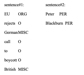
Four types of named entities are concentrated: person (PER), location (LOC), organization (ORG) and names of miscellaneous entities (MISC) that do not belong to the previous three groups. All the other tokens not belonging to the four named entities are labeled as O.
Data are split to train dataset with 14041 sentences, development dataset with 3250 sentences and test dataset with 3453 sentences. Since the labels of the test sentences are not given, we use the development dataset as the test dataset, and divide the train dataset into train and development dataset according to 0.8 vs 0.2 ratio.
Examples of sentences and labels are:
Training Procedures
We concentrate on five models: FNN, BNN, EBNN, RNN [16] and GRU[17]. for FNN, BNN and EBNN models, each sentence is windowed using window size \(w=1\), there are altogether 203621 and 51362 windowed inputs for training and test data, respectively; for RNN and GRU model, the windowed inputs belonging to one sentence are grouped together, resulting in 14041 lists of windowed inputs for training data, 3250 for test data. We define the vocabulary size \(V=20000\) words. In additional to word embeddings as input features. The tunable hyperparameters include ‘batch size’, ‘learning rate’, ‘decay rate’, ‘number of training epoch’, ‘hidden size’. There are two additional hyper parameters to be tuned in BNNs: ‘prior variance for weight’, ‘prior variance for bias’. We use grid search to find out the relatively optimal set of hyperparameters for each of the five models.
During training, we partition the training data into minibatches based on ‘batch size’ and re-weight \(KL(q||p)\) in Equation (8) by \(1/M\) [1][3].
Accuracy Metrics
Because of the unbalanced labels in the dataset (majority of the tokens are O category), we evaluate the results based on the precision and the recall at the entity level fro seqval package.
Results
Accuracy vs Training Time
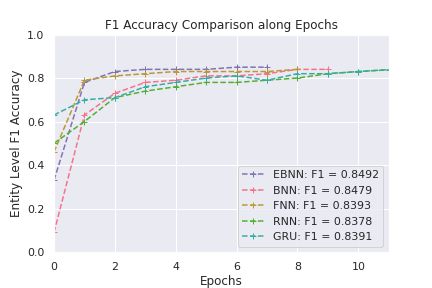
Models are compared in terms of F1 accuracy and training time. Figure 1 shows the F1 accuracy of each model along training epochs. Even though the final F1 accuracies for these five models are close, the accuracy of EBNN, because the prior variance is determined analytically and guaranteed to be the optimal in each epoch, climbs and converges fast; on the opposite, BNN model requires the manual tuning of the prior variance for both weights and biases, it takes BNN some time to reach to the final accuracy. The weights and biases of FNN doesn’t involve distributional assumptions, which means there are only half of the number of model parameters to learn compare to that of EBNN and BNN, FNN is comparable to EBNN in efficiency but slightly lower in F1 accuracy.
Uncertainty of Classification
We computed the prediction uncertainty according to Equation (14) by sampling the model weights for \(S=50\) times, the resulting 50 \(\hat{p}\)’s (each element in \(\hat{p}\) is a vector of estimated probability for 5 classes), are used to compute the measure in Equation (14) for classification uncertainty for each of the five entity classes for each token. Using two sentences from the test dataset, Figure 2 demonstrates the sample standard deviations for the predicted and true label of each token.
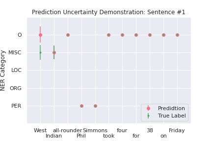
For sentence #1, the first token “West” is classified incorrectly. We can see the estimated uncertainty for both the predicted (pink) and the true (green) labels are relatively large, indicating that the predicted probabilities for these two labels vary a lot across 50 samples, and the model seems to be uncertain in determining the label. For the second token “Indian”, even though the model has uncertainty, its prediction is correct. For the other tokens in this sentence, the uncertainty is almost 0, meaning that the predictions are made confidently.
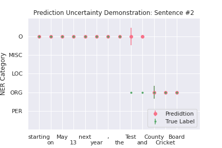
For sentence #2, “Test” and “and” are predicted wrongly. Again, the uncertainty for predicting “Test” as O seems big, but the model is relatively certain that the label should not be “ORG” because the uncertainty level for “ORG” for token “Test” is almost 0. Further, the model is pretty certain to predict “and” to be “O” rather than “ORG”, which conforms to people’s intuition and perception.
Conclusions
In this study, we apply EBNN to classification problem in NLP area, which is an under-explored area. Results show that, for the named entity recognition task, EBNN converges faster and is comparable with other four deep learning models, in addition, EBNN provides the measure for inference uncertainty, which is informative especially for the wrong predictions.
[1] Blundell, Charles, et al. “Weight uncertainty in neural networks.” arXiv preprint arXiv:1505.05424 (2015).
[2] Neal, Radford M. “Bayesian learning via stochastic dynamics.” Advances in neural information processing systems. 1993.
[3] Wu, Anqi, et al. “Deterministic variational inference for robust bayesian neural networks.” arXiv preprint arXiv:1810.03958 (2018).
[4] Nickisch, Hannes, and Carl Edward Rasmussen. “Approximations for binary Gaussian process classification.” Journal of Machine Learning Research 9.Oct (2008): 2035-2078.
[5] Rasmussen, Carl Edward. “Gaussian processes in machine learning.” Summer School on Machine Learning. Springer, Berlin, Heidelberg, 2003.
[6] Lee, Jaehoon, et al. “Deep neural networks as gaussian processes.” arXiv preprint arXiv:1711.00165 (2017).
[7] Cho, Kyunghyun, et al. “Learning phrase representations using RNN encoder-decoder for statistical machine translation.” arXiv preprint arXiv:1406.1078 (2014).
[8] Jaakkola, Tommi S., and Michael I. Jordan. "Bayesian parameter estimation via variational methods.
[9] Graves, Alex. “Practical variational inference for neural networks.” Advances in neural information processing systems. 2011.
[10] Krishnan, Rahul G., Uri Shalit, and David Sontag. “Deep kalman filters.” arXiv preprint arXiv:1511.05121 (2015)." Statistics and Computing 10.1 (2000): 25-37.
[11] Hinton, Geoffrey E., and Drew Van Camp. “Keeping the neural networks simple by minimizing the description length of the weights.” Proceedings of the sixth annual conference on Computational learning theory. 1993.
[12] Kwon, Yongchan, et al. “Uncertainty quantification using bayesian neural networks in classification: Application to ischemic stroke lesion segmentation.” (2018).
[13] Kwon, Yongchan, et al. “Uncertainty quantification using Bayesian neural networks in classification: Application to biomedical image segmentation.” Computational Statistics & Data Analysis 142 (2020): 106816.
[14] Shridhar, Kumar, Felix Laumann, and Marcus Liwicki. “Uncertainty estimations by softplus normalization in bayesian convolutional neural networks with variational inference.” arXiv preprint arXiv:1806.05978 (2018). [15] Sang, Erik F., and Fien De Meulder. “Introduction to the CoNLL-2003 shared task: Language-independent named entity recognition.” arXiv preprint cs/0306050 (2003).
[16] Cho, Kyunghyun, et al. “Learning phrase representations using RNN encoder-decoder for statistical machine translation.” arXiv preprint arXiv:1406.1078 (2014).
[17] Goller, Christoph, and Andreas Kuchler. “Learning task-dependent distributed representations by backpropagation through structure.” Proceedings of International Conference on Neural Networks (ICNN’96). Vol. 1. IEEE, 1996.
Author Luyao Peng
LastMod 2020-09-04